Constructing Flats

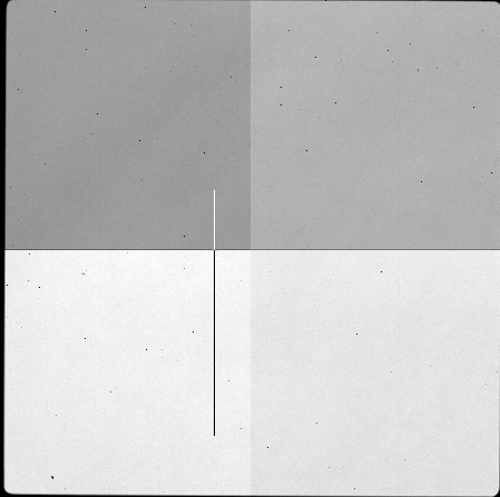
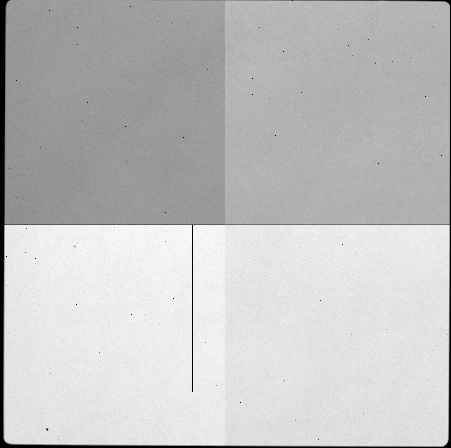
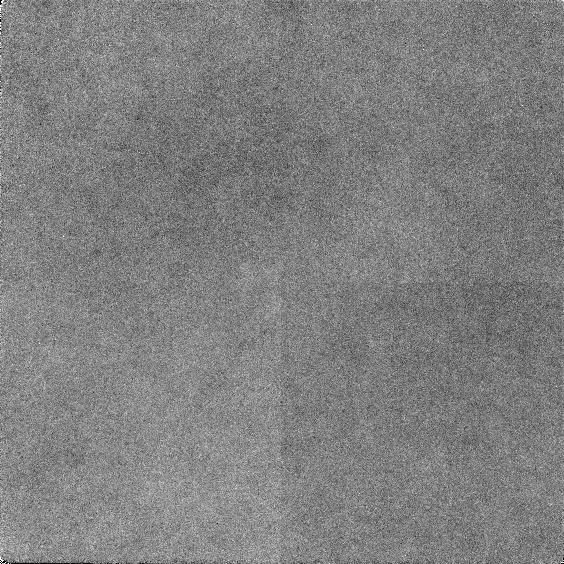
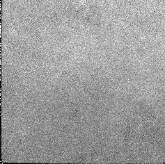
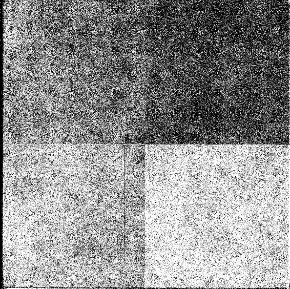
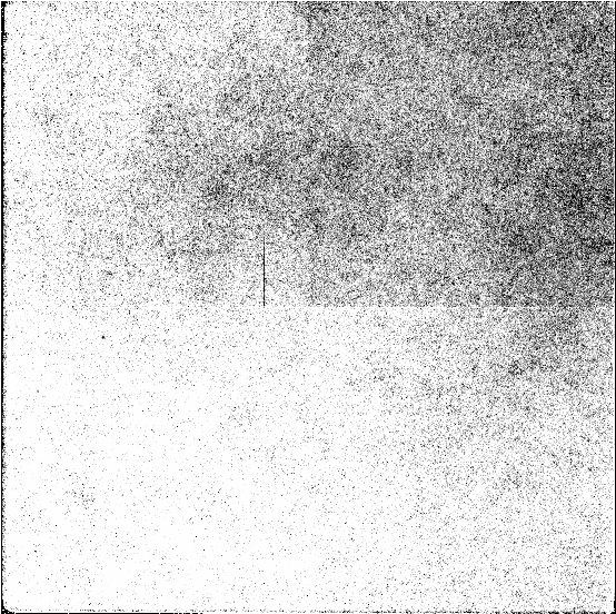
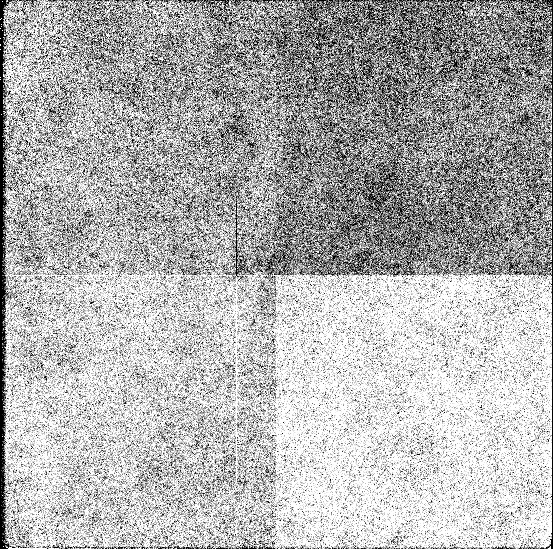
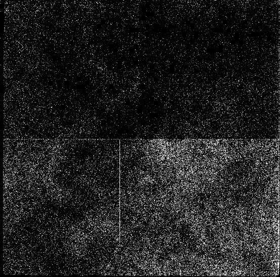
For an effective flat field, we want an image of uniform brightness. For these observations, we have images of the sky taken at twilight. After basic reductions, we combine these twilight images into a master flat for each night using imcombine in IRAF. To normalize these master flats, we use imarith to divide the image by the mean value (found using imstat). Here's an example of a normalized flat from December 9th:

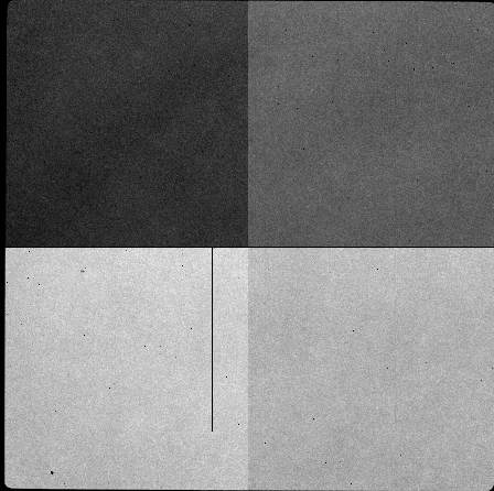
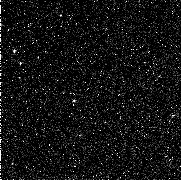
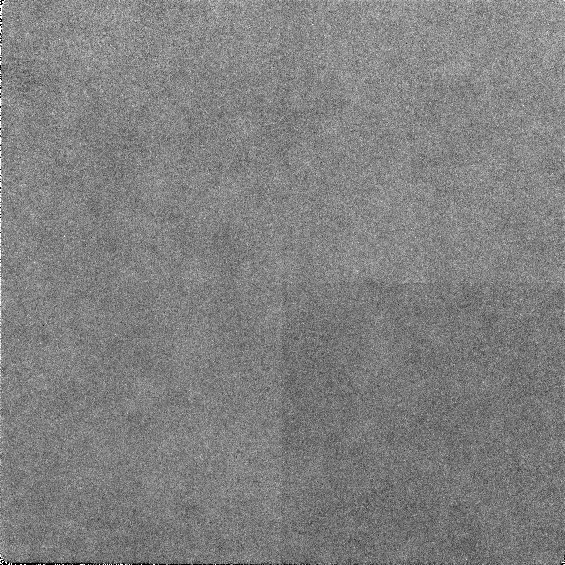
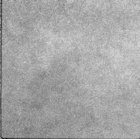
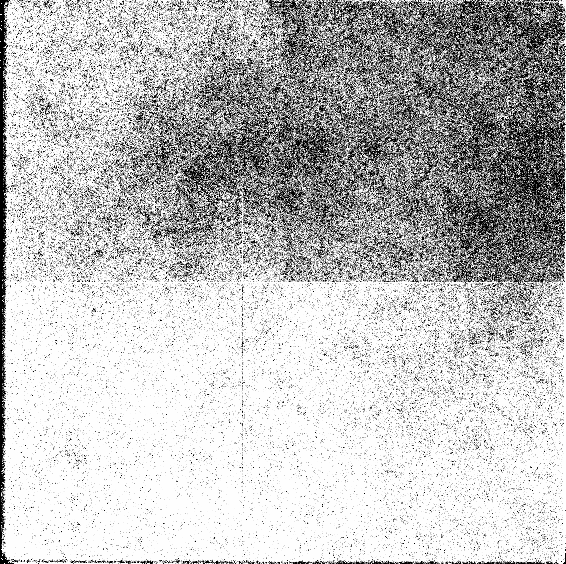
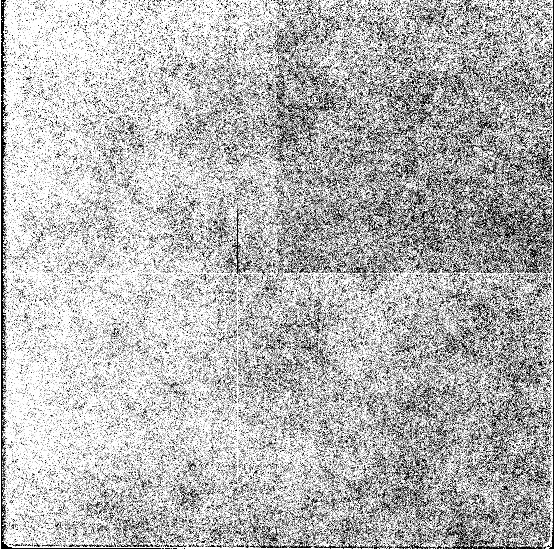
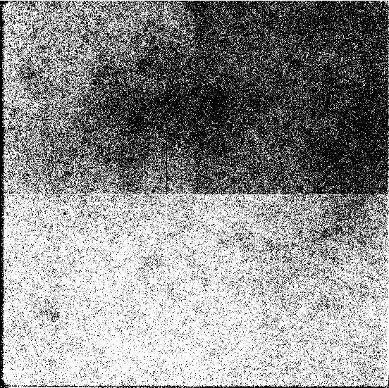
However, these twilight images could have some gradient or other types of non-uniformity. Since the pointings around the Crab are relatively sparse fields, we may be able to use them as sky images. The idea is that if we divide all the Crab field pointings by each other, the individual stars should come out. The only problem is that some fo the fields can be dense, so the odds are likely that two stars would line up even if they're completely different objects. Using only the long exposures (900 seconds) of the Crab fields, we can produce a Crab flat. This is an example from December 11th:

There are no obvious stars left behind, but we're still seeing the diffuse regions of the individual star profiles left over. This is normal and expected. The counts do no hover around 1 because this frame has not yet been normalized.

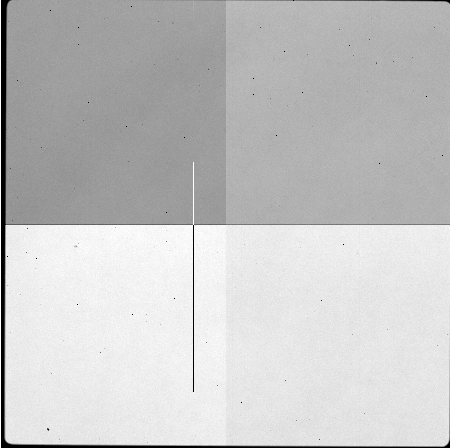
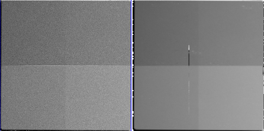
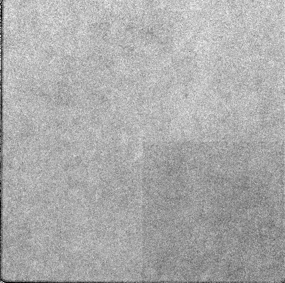
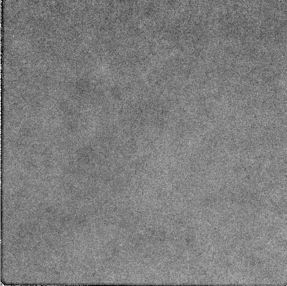
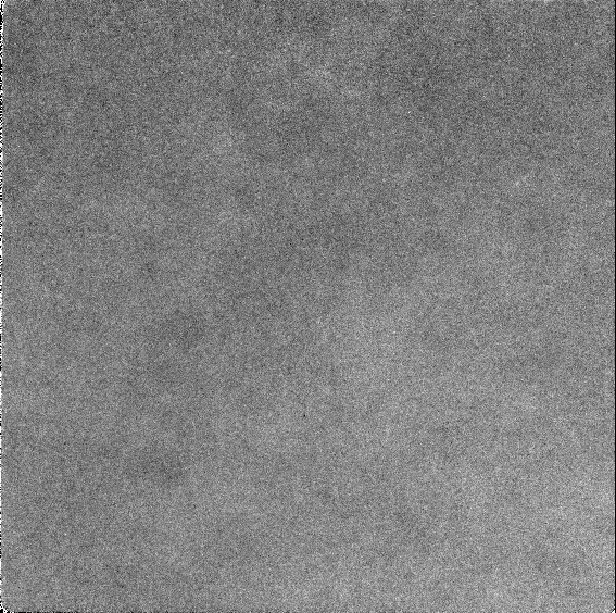
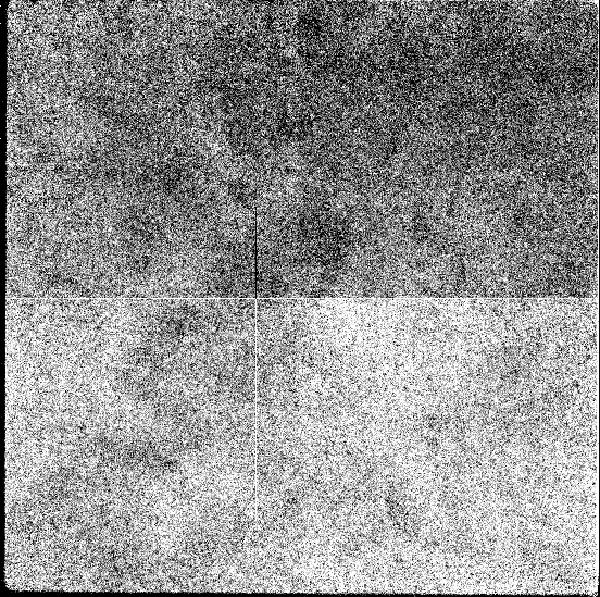
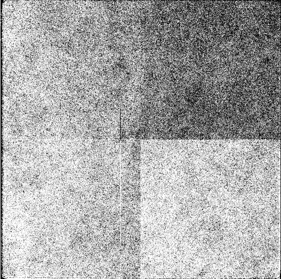
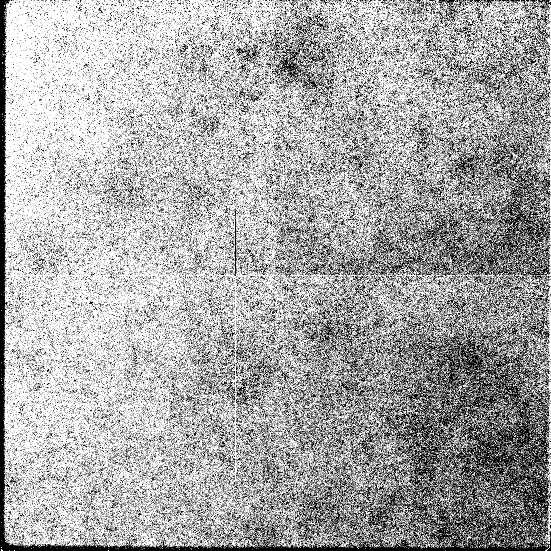
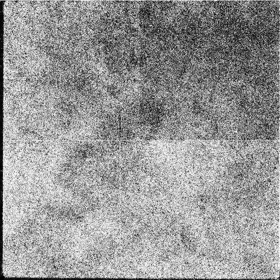
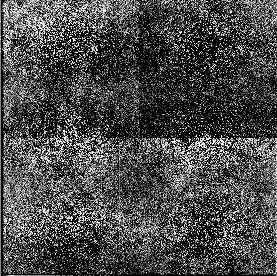
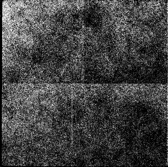
Once normalized, I can combine all my twilight flats and Crab field flats into Master flat images. Since I normalized every frame, the combined images should still have a mean value of 1.  I now have both MasterCrab and MasterFlat images.

There is a gradient in the twilight flats, but not in the Crab flats.  There are also differences in sensitivity depending on the quadrant of the CCD, as they are not all read by the same circuit.  It could prove useful to obtain averages and standard deviations of each quadrant, labeled here:

We can measure each quadrant by using imstat in IRAF.  For example, statistics for quadrant 4 are obtained using

imstat masrat[200:1800,200:1800]

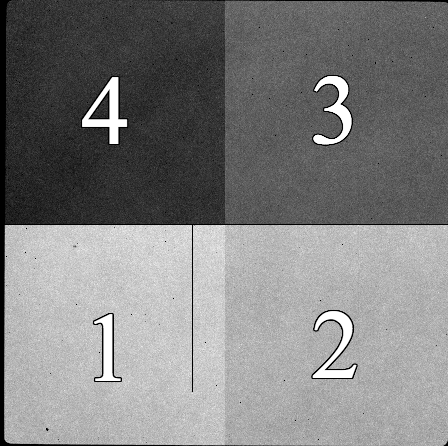
Quadrant	Mean	Std. Dev.
4	0.9871	0.004252
3	0.9831	0.003526
2	0.9869	0.003893
1	0.99	0.003072

We can use these average values to construct a Sky Correction flat called SkyCorr.  To do this, we use artdata's mkpat command to create a 4072x4064 (resolution of the ccd) image full of zeros.  We then replace the values in each quadrant with the mean values in the above table by entering imreplace SkyCorr[x1:x2,y1:y2] <1/mean value>, where the coordinates are the limits of the quadrant.  The result looks like this:

This looks like you'd expect judging by the table.  Indeed, quadrant 3 is the brighest and quadrant 1 is the dimmest (remember, this is the inverse value, so the ranking is also reversed).

Now, you're probably wondering why we've used the inverse mean.  This is because the way we're flattening the images.  More explicitly,

imarith <llzimage> / MasterFlatn tmp
imarith tmp / SkyCorr fllzimage

We now have a flattened, linearity corrected, line biased, and zeroed image.  Had I used MasterCrab/MasterFlat to get the averages, then the simple mean would have been fine for constructing the SkyCorr image.  Since I did the inverse of that, we take the inverse of the mean.

And now a look at what all this hard work has done:

This is a flattened image of SA 92, one of our Landolt standard fields.

Updated June 2013