Rotation Curve Fitting
Traditionally, we fit ellipses to the images to obtain an azimuthally averaged surface brightness profile (the solar luminosity per square parsec as a function of radius along the major axis of the ellipses). [I say traditionally because it is now possible to use the full 2D information with programs like DISKFIT rather than azimuthally averaging around each ellipse.] The surface brightness profile is corrected to face-on for a measured inclination and a guess as to what the galaxy would look like edge-on. (i.e., we usually assume some finite thickness for the galactic disk. However, real disks are observed to be pretty thin, about 8:1 on average, so simply assuming a thin disk [S(r) = sobs(r)/cos(i)] is already pretty good.)
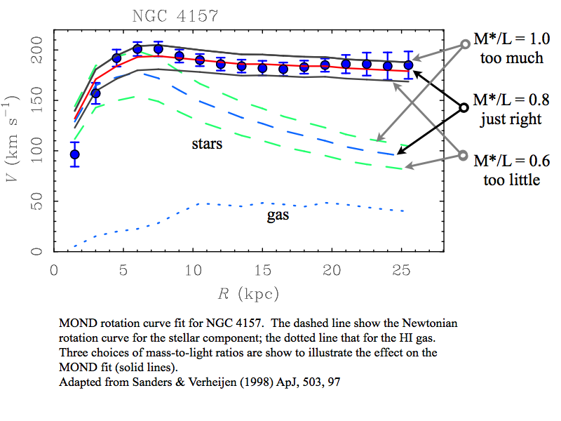
The face-on surface brightness profile is converted to a mass surface density profile assuming a mass-to-light ratio for the stars. This is later treated as a fit parameter - we do not know M*/L a priori. For the HI gas, this conversion is known (there is no free parameter). Most galaxies are treated as two components, a thin disk of stars plus a thin disk of gas. Some additionally have a central bulge component which might be treated as a 3D blob of stars with a separate M*/L from the disk.
From the mass surface density profile, the Poisson equation is numerically solved to obtain the rotation curve predicted by each component: stars and gas. i.e., for the observed distribution of stars, Newton predicts we should observe V*(r), and the same for the gas Vg(r). There are tasks in the GIPSY package to do this. [If you wish to write your own, read up on it first to save yourself from rediscovering some numerical traps.]
[Note: masses add linearly, and M ~ r*V^2, so at a given radius, velocities add in quadrature.]
We now have a Newtonian mass model for the observed baryonic components: Vb^2(r) = V*^2(r) + Vg^2(r).
So far, the procedure I have described is perfectly conventional - the same is done whether we wish to consider dark matter or MOND.
In the case of dark matter, the observed velocity V^2(r) = Vb^2(r) + V_DM^2(r). Anything we canât explain with the baryons we attribute to dark matter. One can fit various halo models to V_DM^2(r) = V^2(r) - Vb^2(r).
In MOND, we instead apply the MOND formula, including the interpolation fcn mu(x) with x = a/a0 and a = V^2/r. We then have V^2(r) = Vb^2(r)/mu(x) Effectively, MOND is an amplification factor [1/mu(x) >= 1] that maps from the rotation curve predicted by Newton to that actually observed.
In order to start doing this, one had to guess at M*/L in order to compute V*(r). We iterate the value of M*/L to ring the best fit. This is quite simple: V*,new(r) = [V*,guess(r)]*sqrt[(M*/L,new)/(M*/L,guess)]. It is also strictly limited: the predicted shape of V*(r) is fixed; the only thing the fit can do is scale it up and down.