Making the Galaxy

1. What is the comoving radius of a sphere that contains enough mass to make the Milky Way?
   I.e., how much of the average density of the universe do you have to scoop up to make our Galaxy?
2. What is the overdensity Δ = ρ/ρ_crit within R = 20 kpc (the approximate edge of the Galactic disk)?
3. Assuming the rotation curve remains flat beyond the edge of the disk, estimate R₂₀₀ & M₂₀₀.
4. Another way to estimate halo masses is abundance matching. What is M₂₀₀ for a galaxy with the stellar mass of the Milky Way according to Fig. 17 of Kravtsov et al.?
   Read off a value for both the Kravtsov relation and that of Moster/Behroozi. How do these abundance matching halo masses compare to your dynamical estimate?
   ASTR 433 only:
5. Use this Milky Way model to make a revised estimate of R₂₀₀. How does it change from the previous answer? Does this improve consistency with abundance matching?

Milky Way data: M_* = 6.2 x 10¹⁰ M_☉; M_g = 1.2 x 10¹⁰ M_☉; V(R=20 kpc) = 213 km/s.
Twenty kpc is the practical edge of the Galactic disk. The dark matter halo extends much further out.

Assume a vanilla ΛCDM cosmology with Ω_m = 0.3, Ω_Λ = 0.7, Ω_b = 0.05, and H₀ = 70 km/s/Mpc.

Hint: think carefully about which cosmic density applies to which part of this problem.

Mass Models

First, subtract off the rotation due to the luminous stars and gas. Whatever is left we call dark matter.

[Hint: Velocities add and subtract in quadrature. Real data are messy. Don't get hung up on tiny inconsistencies: deal with them.]

1. Fit the data with both a pseudo-isothermal halo and a NFW halo. Plot the results. Does either model provide a better fit?
   
2. A specific choice of the B-band stellar mass-to-light ratio is provided in the data file. This is rather uncertain, so repeat (i) using M_*/L = 0.5 for both bulge and disk components.
   [Hint: How does velocity scale with M/L?]
3. In the NFW case, what is the escape velocity for a star at r = r_s?
   [Recall: V_esc² = 2 |Φ(r)|.]
4. Does the escape velocity seem well determined? Why did I not ask for the total mass of each halo? Or for the escape velocity of the pseudo-isothermal halo?

Halo Mass and Concentration

1. Plot theory and data together.
   Include a band of width 0.11 dex in log(concentration) to represent the intrinsic scatter in the halo mass-concentration relation.
   The quantity V₂₀₀ is reported for the data; this is equivalent to halo mass since mass scales as the cube of circular speed: M₂₀₀ = 3.3 x 10⁵ (V₂₀₀)³ for units in solar masses and km/s.
2. Interpret the plot.
   Note that the signature of the cusp-core problem is that NFW fits result in very low concentrations and high R₂₀₀. This happens because a fitting algorithm will attempt to approximate the linear rise of the rotation curve of a halo with a constant density core by stretching out the NFW form, as any function looks linear if one zooms in enough.

Tully-Fisher and M_*/L

Use the SPARC data provided here to answer this question.

1. Construct the Tully-Fisher relation. Plot the 3.6 micron luminosity against the flat rotation velocity and fit it with a straight line in log space:
   log₁₀(L₃₆) = X log₁₀(V_f) + K
   where X is the slope and K the intercept of the Tully-Fisher relation.
   Report the fitted values of X and K along with their uncertainties and show the fitted line on the plot with the data.

   Consider two cases: all the data with a measured flat rotation velocity, and a high quality subset that have distance uncertainties less than 20% and Q < 3 (Q = 3 are lousy rotation curves).

   Are the data well fit as a straight line? What differences do you notice between the high quality subsample and the entire sample?
   [Recall that for base 10 logarithms, the uncertainty δu in variable u transforms to 0.43(δu/u) in log₁₀(u).]

2. Construct the baryonic Tully-Fisher relation,
   log₁₀(M_b) = X log₁₀(V_f) + K
   where the baryonic mass is the sum of stellar and gas mass:
   M_b = M_*+M_g = 0.5(L₃₆−L_bulge)+0.8L_bulge+1.4M_HI.
   Note that this formula assigns a mass-to-light ratio of 0.5 to the disk, 0.8 to the bulge, and the gas masses is corrected to include helium by multiplying by 1.4. The disk lumminosity is computed by subtracting the bulge light from the total.

   Consider two cases above: all the data with a measured flat rotation velocity, and a high quality subset that have distance uncertainties less than 20% and Q < 3.

   Are the data well fit as a straight line? What differences do you notice between the high quality subsample and the entire sample?

3. Now reverse the problem. Given a baryonic Tully-Fisher relation with parameters X = 4 and K = 1.7, compute the mass-to-light ratio of each galaxy. Plot a histogram of M_*/L for the two samples. Do the results seem reasonable?
   Also plot M_*/L against L/M_HI. What is the threshold where gas and stellar mass are equal? What happens as you cross this threshold?

   ASTR 433 only:

4. How does the baryonic Tully-Fisher relation change if we double the mass-to-light ratio to 1.0 for the disk and 1.6 for the bulge? If we halve it to 0.25 and 0.4? Do these changes result in a simple translation of the intercept? Or is the slope also affected? Why?

There is an explanatory note at the bottom of the data file describing each column. Be sure you understand the meaning of the relevant columns and their physical units (e.g., luminosities are given in billions of solar luminosities). You will need to plot the data, fit it, and be able to select subsets of the data as indicated. I encourage you to use Python, but I don't want to see your code, just the results with a cogent discussion.

Virial Temperature

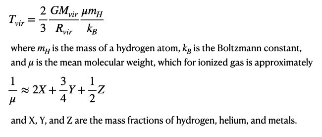
1. What is the virial temperature of a typical Milky Way-size galaxy with a virial mass of 10¹² M_☉ and radius of 200 kpc?
   Assume a primordial gas with X=3/4, Y=1/4, Z=0.
2. Now consider a solar composition (X = 0.7, Y = 0.28, Z = 0.02) gas. What changes? How much difference does this make?

   Look at the cooling rates in Figure 1 of Benson (2010).

3. Where does our object sit on the primordial cooling curve?
   Milky Way-mass galaxies are thought to be the most efficient at turning gas into stars. Does this follow from your answer here?
4. Now consider the solar metallicity cooling curve in Benson's figure. By what factor does the cooling rate change relative to the primordial case? [Read numbers off the graph to find their ratio.]
   Comment on how this might affect the efficiency of star formation.
   Given these considerations, does it make sense for star formation to be more efficient in the early, low metallicity universe as implied by JWST observations of bright, high redshift galaxies?